Examples of plotting TrackRun subsets

Import the necessary modules

Note Examples below require cartopy package to be installed

import cartopy
import cartopy.crs as ccrs
import matplotlib.pyplot as plt
from pathlib import Path
import xarray as xr

from octant.core import TrackRun, OctantTrack

To save time, in this example lcc_map function is used to create a map in Lambert Conformal Conic projection.

def lcc_map(fig, subplot_grd=111, clon=None, clat=None, coast=None, extent=None):
    """Create cartopy axes in Lambert Conformal projection."""
    proj = ccrs.LambertConformal(central_longitude=clon, central_latitude=clat)

    # Draw a set of axes with coastlines:
    ax = fig.add_subplot(subplot_grd, projection=proj)
    if isinstance(extent, list):
        ax.set_extent(extent, crs=ccrs.PlateCarree())
    if isinstance(coast, dict):
        feature = cartopy.feature.NaturalEarthFeature(
            name="coastline", category="physical", **coast
        )
        ax.add_feature(feature)
    return ax

Some useful declarations for plotting…

plt.rcParams["figure.figsize"] = (15, 10)  # change the default figure size
COAST = dict(scale="50m", alpha=0.5, edgecolor="#333333", facecolor="#AAAAAA")
clon = 10
clat = 75
extent = [-20, 50, 65, 85]
LCC_KW = dict(clon=clon, clat=clat, coast=COAST, extent=extent)

mapkw = dict(transform=ccrs.PlateCarree())

Define the common data directory

sample_dir = Path(".") / "sample_data"

Data are usually organised in hierarchical directory structure. Here, the relevant parameters are defined.

dataset = "era5"
period = "test"
run_id = 0

Construct the full path

track_res_dir = sample_dir / dataset / f"run{run_id:03d}" / period

Load the data

Load land-sea mask array from ERA5 dataset:

lsm = xr.open_dataarray(sample_dir / dataset / "lsm.nc")
lsm = lsm.squeeze()  # remove singular time dimension

Now load the cyclone tracks themselves

tr = TrackRun(track_res_dir)

tr

Cyclone tracking results
Number of tracks	671
Data columns	lon, lat, vo, time, area, vortex_type
Sources
	sample_data/era5/run000/test

conditions = [
    ("long_lived", [lambda ot: ot.lifetime_h >= 6]),
    (
        "far_travelled_and_very_long_lived",
        [lambda ot: ot.lifetime_h >= 36, lambda ot: ot.gen_lys_dist_km > 300.0],
    ),
    ("strong", [lambda x: x.max_vort > 1e-3]),
]

tr.classify(conditions)

… and classify them

What are the indices of “strong” cyclones?

tr["strong"].index.get_level_values("track_idx").unique()

Int64Index([93, 182, 252, 569, 631], dtype='int64', name='track_idx')

Simple track plot

Select an OctantTrack by its absolute index

import pandas as pd

random_track = tr["strong"].loc[182]

Here the variable random_track is a subclass of pandas.DataFrame, and it has the following additional attributes and methods:

set(random_track.__dir__()).difference(set(pd.DataFrame().__dir__()))

{'area',
 'average_speed',
 'coord_view',
 'from_df',
 'from_mux_df',
 'gb',
 'gen_lys_dist_km',
 'lat',
 'lifetime_h',
 'lon',
 'lonlat',
 'lonlat_c',
 'max_vort',
 'plot_track',
 'time',
 'total_dist_km',
 'tridlonlat',
 'tridlonlat_c',
 'vo',
 'vortex_type',
 'within_rectangle'}

One of them is plot_track() method, which is a small wrapper around matplotlib.pyplot.plot() function.

The important (optional) parameter is ax=, via which a track can be plotted in the given axes. For example, below a figure fig is created along with ax, geo-referenced axes, and then the chosen track is added to the plot. The remaining parameters that can be passed to plot_track are keyword arguments of matplotlib.pyplot.plot(*args, **kwargs) function.

Plot a single track on a map

fig = plt.figure()
ax = lcc_map(fig, **LCC_KW)
random_track.plot_track(ax=ax, color=None);

Plot a single track without a map

a) In the given Axes

fig, ax = plt.subplots()
random_track.plot_track(ax=ax);

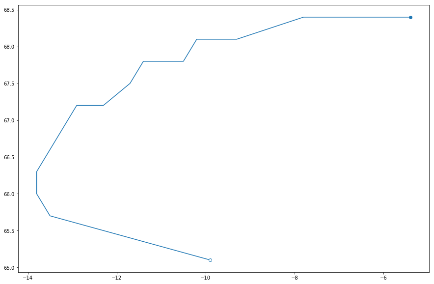
b) Or automatically create figure and axes in the PlateCarree projection

random_track.plot_track();

The function returns matplotlib axes object, so it can be used for further plotting.

ax1 = random_track.plot_track(color='xkcd:stormy blue',
                              linewidth=3,
                              label=f'track 3317')
ax1.legend(loc=4)
ax1.set_title('My plot');

Plot all tracks from TrackRun

subsets_and_colors = [("long_lived", "#424242"), ("far_travelled_and_very_long_lived", "C0"), ("strong", "C1")]

fig = plt.figure()
ax = lcc_map(fig, **LCC_KW)

handles, labels = [], []
for subset_label, color in subsets_and_colors:
    for (_, track) in tr[subset_label].gb:
        track.plot_track(ax=ax, color=color, label=subset_label)

labels, handles = [
    list(getattr({j: i for i, j in zip(*ax.get_legend_handles_labels())}, m)())
    for m in ["keys", "values"]
]
ax.legend(handles, labels, fontsize="x-large", loc=1);